Introduction

Machine learning is one of the hottest topics in tech today. In this article, I will explain what is meant by machine learning, and how gradient descent works.

Let's get right into it.

Traditional Programming Vs Machine Learning

Traditional Programming

In traditional programming, a developer has to write a set of rules which the computer has to follow to perform a certain task.

For example, assume we want to write a very simple program that takes a number (x) as its input and multiplies it by 2, and then adds 10. For this problem, we would have to define a function such that y = 2x+ 10.

In this function, the user will provide the input x which can be any number, and the program will return the output y.

Pretty simple, right?!

The above function has 3 components:

1. The input features

   In this case, we have a single input feature, x.

2. The output (y)

3. The parameters that map the input (x) to the output (y)

   In the above function, we have two parameters, 2 (coefficient) and 10 (intercept).

   You can think of parameters as the rules that map the input to the output. Because the above function is simple, we were able to figure the rules out ourselves.

Machine Learning

Now, consider the following scenario.

You were asked to write a program that estimates the prices of houses in a certain area using specific features of the houses such as the area of the property, the location, the number of rooms, etc.

Again, such a program will have 3 components:

1. The input features

   In that case, let's say there are 10 input features (x_1, x_2, …., x_10) representing different properties of each house.

2. The output target

   The price of the property.

3. The parameters (rules) that map the input features to the output target

   Because the above problem is infinitely more complicated than the previous one, it is almost impossible to figure out the parameters ourselves.

   This is where machine learning shines.

Machine learning is used in complex problems for which using traditional approaches yield no good solutions, or require a lot of tuning and maintenance.

In machine learning, instead of us writing the rules for the computer to follow, we only provide the computer with the input features and the expected output. The computer will then use certain algorithms to understand the underlying structure of data and learn the parameters (rules) that describe the relationship between the input features and the output.

So the goal of machine learning is to build and train models to learn the parameters that map the inputs to the outputs and then make accurate predictions on new data it has not seen before.

One of the most common algorithms for training machine learning models is called Gradient Descent.

Gradient Descent

Gradient descent is an iterative optimization algorithm that was introduced in 1986 by David Rumelhart, Geoffrey Hinton, and Ronald Williams, when they published their groundbreaking paper "Learning Internal Representations by Error Propagation".

Gradient descent aims to find the optimal parameter values by tweaking them iteratively.

For the sake of simplicity, let's consider the following function with a single parameter y = θ x.

This function contains the input x, the output y, and a single unknown parameter θ (theta).

As discussed above, we will provide the gradient descent algorithm with both the input and output values, and it will learn the parameter θ by itself.

How would it do that?

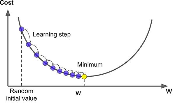
1. We start by giving the parameter θ a random value. This is called random initialization.

2. Next, we use the randomly initialized parameter to compute our predictions. predictions = θ x.

   Because θ is randomly initialized, we can expect the predictions to be very different from the actual output values.

3. We then compute a function that measures the distance between our predictions and the actual output. This function is called a cost function which basically computes how bad our model is performing.

   We need to find the optimal value of the parameter θ to compute the best possible predictions, hence minimizing the cost function.

   So our goal is to tweak the model parameters iteratively until we converge to the minimum value of the cost function.

4. After computing the cost function, this is when calculus kicks in. We measure the gradient of the cost function with regard to the current value of θ.

   Without getting into too much math, calculating the gradient allows us to know how θ should be tweaked in order to maximize the cost function, which is the opposite of what we really want.

   So after calculating the gradient, we update the parameter θ by subtracting the gradient from the current value of θ.

   Notice that we subtracted, instead of added the gradient because we want to minimize the cost function.

   θ = θ - η * dθ

   dθ is the gradient of the cost function with regard to θ, and η is the learning rate (will be discussed below).

5. Now with the new value of θ, we compute the predictions and the cost function once again.

   We can expect more accurate predictions and a lower cost function than the previous iteration. However, this is probably not the lowest possible value for the cost function.

6. We update the value of θ once again as in step (4) using the new value of the cost function, and repeat the cycle until we converge to the minimum possible value of the cost function (global minimum).

So we update the value of θ gradually, taking one gradient descent step at a time, each step attempting to minimize the cost function.

Keep in mind that as the cost function decreases with each step, the gradient also decreases, so the steps gradually get smaller and smaller as you approach the global minimum.

You can see that the gradient descent algorithm works by measuring the gradient of the cost function with respect to each model parameter, and then moves in the direction of descending gradient. Once the gradient is zero, you have reached a minimum.

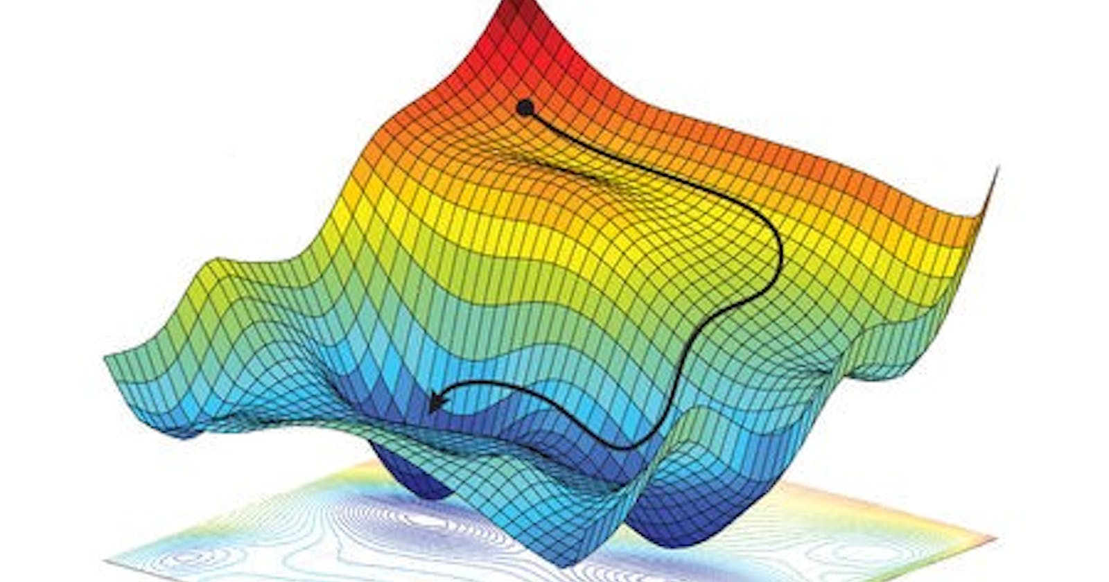
Note that in the above example, the problem was very simple as we were dealing with a limited one-dimensional parameter search space. In real-world projects, models will have much more parameters, and gradient descent will be searching through a much higher dimensional parameter space.

Learning Rate (η)

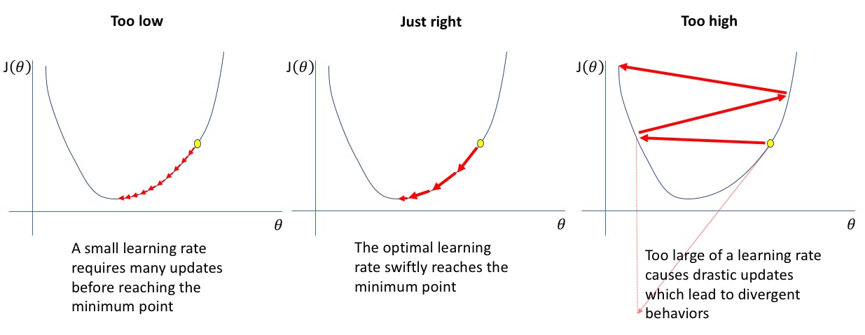
The learning rate is a hyperparameter that determines the size of each gradient descent step.

If the learning rate is too small, then the algorithm will have to go through many iterations before converging to the global minimum, which ultimately results in a longer training time.

However, if the learning rate is too high, the algorithm could diverge away from the global minimum.

Parameters Vs Hyperparameters

As discussed above, model parameters represent the rules that the learning algorithm needs to learn to map the input features to the output values to make accurate predictions.

A hyperparameter, however, is a parameter of the learning algorithm, not of the model itself. It must be set before training, and it is not affected in any way by the learning algorithm, so it remains constant during training.

Hyperparameters, such as the learning rate, are used to control the learning process. When training machine learning models, you should experiment with different values for each hyperparameter until you find the best value. This process is called hyperparameter tuning.

Summary

1. Machine learning is used in problems that can not be approached using traditional techniques.
2. Machine learning allows programs to learn without being explicitly programmed.
3. The goal of training machine learning models is to find the optimal parameter values that best describe the relationship between the input features and the output values.
4. Gradient descent is one of the most common machine learning algorithms which aims to find the best parameter values by minimizing a cost function.
5. Training machine learning models is an iterative process whose rate depends on the learning rate, the number of model parameters, etc.